So you are looking to digitalize some aspects of your materials R&D, and you know that molecular dynamics, or MD for short, is one approach. But what are its strengths and weaknesses and which variant should you turn to? In this text I will give you a brief primer.
What is Molecular Dynamics?
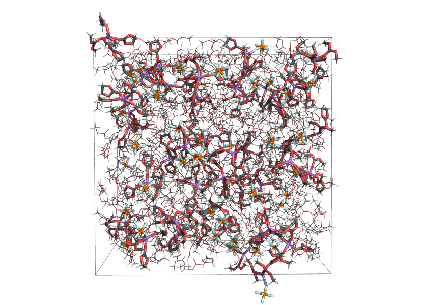
Molecular dynamics (MD) is an approach to modeling materials that involves simulating the motions of atoms and molecules by computing the forces on each according to some model for the interactions between them. Most often, the question is reformulated as computing the system’s potential energy surface (PES) in terms of its atomic coordinates, from which the force on an atom is recovered as the gradient of the PES upon moving that atom. From some starting point of a system contained in a simulation box, typically on the nanometer scale, the system can be propagated in time by updating positions and velocities based on the computed forces. This process generates a trajectory of the system, consisting of the positions and velocities of each atom at each time step.
The real power of MD comes not from the trajectories themselves, but from the material properties that can be extracted from them by means of statistical mechanics: ionic conductivity, density, species diffusivities, local and global structure and structural dynamics, etc.
To illustrate the connection between trajectories, statistical physics and material properties, let me give a representative example. You may be interested in the diffusivity of a species in a solution. Fick’s theory of diffusion tells us that species diffuse in the direction of decreasing concentration, with the proportionality constant being the (self-)diffusivity. Intuitively, one might therefore expect that we would need to set up a concentration gradient in order to compute the diffusivity from an MD simulation. However, Einstein established a connection between Brownian motion (i.e. random walk) and diffusion which also explains why diffusion occurs: it’s not that species “want to” eliminate concentration gradients, that is just a consequence of the random motion resulting from the interactions of an atom with all others.
This can be understood by considering a series of coin flips where we compute the number of heads minus the number of tails. The average difference across several series will be zero since there is an equal chance of there being more heads or more tails. However, the expectation value for the square of the difference is nonzero and grows linearly with the number of steps, where again the constant of proportionality is the diffusivity. Once we have computed the diffusivities of all species, we can also compute other properties such as ionic conductivity by different statistical physics relations, without the need for an explicit electric field.
Most often MD simulations are applied to bulk systems, where surface effects are eliminated by making the simulation cell periodic in all directions. In general, any material properties that can be understood in terms of the interactions of atoms and molecules in a simulation box can be studied using MD. The most relevant caveats have to do with limits on time and length scales. Most properties can be computed without adding gradients or transients to the simulation, but the latter is also common practice, and known as non-equilibrium MD (NEMD). Depending on your system and selected approach, MD simulations may be used to predict among other properties:
- Density
- Viscosity
- Mechanical strength and stiffness
- Ionic conductivity
- Dielectric constant
- Local and global structure
- Lifetimes of bonds and structures
- Chemical reactions
- Diffusivities
- (partial) vapor pressure
- Phase diagrams
- Entropy
Why do we need different MD methods?
The main reason we need more than one MD method, is that we need to make approximations to the physics. To quote Paul Dirac:
“The underlying physical laws necessary for the mathematical theory of the whole of chemistry are thus completely known, and the difficulty is only that the exact application of these laws leads to equations much too complicated to be soluble.”
Although this quote was given almost a century ago, it remains true to this day. We know that we in principle need to solve the time-dependent Schrödinger equation for the many-body wave function of all atomic nuclei and electrons in the system, which is a function of as many dimensions as there are nuclei and electrons in the system times three; a completely intractable problem for all but the smallest systems.
MD methods can be classified into a rough taxonomy based on how big approximations they make to the exact physics, and concomitantly how big systems they can handle at practical computational cost.
The exact time-dependent Schrödinger equation is almost never solved in practice in MD simulations. Instead, the first approximation is typically the Born-Oppenheimer approximation; that electronic motion is orders of magnitude faster than nuclear motion so that the problems of electronic and nuclear motion can be handled separately. This will be assumed in all the following sections, which start from the most exact approaches and then treat increasing levels of approximation.
Ab Initio MD
Ab initio MD (AIMD, ab initio from lat. “from first principles”) refers to MD methods using density functional theory (DFT) for evaluating energies and forces. DFT is an in principle exact theory that states that the ground state energy and wave function of a system of electrons is uniquely determined by the electron density, which reduces the dimensionality from 3N to 3. Unfortunately, the mapping, or density functional, is not exactly known, and thus approximations are needed. There is a wide range of DFT functionals, of which PBE is a popular choice for MD, based on the local density and its first derivative.
In addition to the approximation involved in selecting a density functional, AIMD is almost universally based on treating the nuclei as classical particles and only solving the time-independent rather than the time-dependent Schrödinger equation for the electrons, either assuming them to always be equilibrated, or propagating the electron density classically with a fictitious inertia. Usually only the valence electrons are treated explicitly since they are most relevant for the chemistry. The forces on atomic nuclei are computed by evaluating the derivative of electron energy with respect to moving each nucleus.
AIMD methods are the most accurate, but also the most computationally demanding, and are mostly used for systems of <1000 atoms simulated for single or low double digit picoseconds. Even at this scale, they are normally not practical for computational screening, but rather suited for deep dives into fewer systems. They are a good choice when accurate interactions are more important than time or length scales or sampling multiple systems. A strength of AIMD methods is that they can represent arbitrary dynamics, such as charge transfer and other types of reactions, as opposed to classical MD (see below).
Semi-empirical methods
There are a number of different approaches based on approximating quantum computations and supplementing with pre-computed integrals based on higher order quantum chemical methods and empirical data.
Two main groups of semi-empirical methods are based on making approximations to either DFT or Hartree-Fock theory. The latter is a quantum chemistry method that captures electron exchange exactly (in the sense that the wave function should change sign when two fermions are exchanged) but treats electron-electron interactions in a simplified mean-field sense (i.e. omitting correlated electron motion). The most well-known methods based on DFT are known as density functional tight-binding (DFTB) methods, and the most well-known methods based on HF are the parametric models developed by John Pople, e.g. PM6 and PM7 (I will call them PMX henceforth).
In contrast to DFT and DFTB, HF and PMX compute the energy as functions of the full wave functions instead of only electron densities. These computations involve integrals for different terms in the Hamiltonian, containing either one or two electrons each. The PMX methods neglect all two-electron terms and use approximate equations and tabulated values for the rest.
DFTB methods, on the other hand, are based on Taylor expansions of the energy as a functional of the electron density, expanded around a reference density, which depends on the composition of the simulated system. They are usually further subdivided based on the leading order of the expansion, DFTB2 or DFTB3, where DFTB3 contains a charge correction to DFTB2 that can additionally account for charge-transfer between atoms.
There is also a modification of the DFTB approach known as extended tight-binding (XTB) which is similar to DFTB2 and DFTB3 but also includes correction terms for dispersion and hydrogen bonding. It is on the same order of computational cost as DFTB2 and DFTB3 but typically slightly more accurate. At Compular we use XTB as our default approach to simulating liquid electrolytes, for which we provide automated workflows in our Simulator web application.
Semi-empirical methods strike a good balance between accuracy and computational efficiency for condensed systems, when greater accuracy than that of classical MD is needed, e.g. for systems with high charge concentrations, such as battery electrolytes, but for which there is a need to simulate more or larger systems than practical with AIMD methods. They also share the versatility of AIMD methods, in that they can account for charge transfer and chemical reactions given that they resolve electronic degrees of freedom. A typical scale for semi-empirical methods is on the order of thousands of atoms and tens to hundreds of picoseconds.
Classical MD
In contrast to AIMD and semi-empirical methods, classical MD does not attempt to resolve electronic structure, but simply treats atoms as classical point particles. The parameterizations of classical MD are alternately known as force fields or inter-atomic potentials (I will use force fields henceforth). These are typically based on two categories of interactions: non-bonded and bonded. The non-bonded interactions are typically based on 1) assigning point charges to atoms and 2) fitting polynomial curves to represent Pauli exclusion and dispersion (most commonly using the van der Waals equation). The bonded terms are mostly based on elastic spring models for bond distances and angles, and Fourier expansions for dihedrals (i.e. torsions).
Since classical MD is not based on explicit quantum theory all parameters need to be fit empirically based on some combination of higher order computational methods or empirical data. For accurate simulations, it is necessary to have multiple parameter sets for each element based on their chemical context. For instance, a carbon atom in a carbonyl group has a different set of parameters than a carbon atom in a methyl group. There are a number of openly available force fields for different domains (e.g. OPLS for liquids, CHARMM and AMBER for biological systems, AMOEBA for water). Nevertheless, to handle novel molecules beyond the scope for which a given force field was parameterized, there is often a need to fit additional parameters as an MD user. On the other hand, classical force fields are much less computationally demanding than either AIMD or semi-empirical methods.
One weakness of most forms of classical MD is that they, based on their functional form, cannot support charge transfer or chemical reactions more generally. There are exceptions to this rule, however. Reactive force fields, such as ReaxFF, have some ability to represent these phenomena. In the case of ReaxFF, which is the most well-known example, a bond order is assigned to each bond on the fly, as a function of the bond distance and the elements involved. These approaches are generally more computationally demanding than other classical force fields, but less so than semi-empirical methods. Accordingly, they are also less accurate.
There are also extensions for handling higher order electrostatics, e.g. dipoles induced by atomic interactions. An example of this approach is the APPLE&P force field, developed by Oleg Borodin, which has been successfully applied to diverse systems with high local charge concentrations, including ionic liquids and highly concentrated battery electrolytes.
A commonality between ReaxFF and APPLE&P is that because they are more advanced than conventional force fields, they require a greater number of parameters, and because they have smaller communities of users, they tend to require more parameter fitting from the end user to be used effectively. They are also available in fewer simulation packages.
Typical system sizes and simulation lengths for classical MD are tens of thousands of atoms and hundreds of nanoseconds.
Coarse grained MD
Some systems are too large or complicated even for classical MD methods to handle. In these cases, coarse grained MD approaches (CGMD) can be of use. They typically reduce the number of free particles by handling molecules and monomers as beads (i.e. particles with spatial extension and orientation). The functional forms can vary widely depending on what physics needs to be resolved. CGMD can for example be used in polymeric systems and heterogeneous materials where morphological structure and dynamics are in focus. An example use case is for battery electrodes where active material particles can be treated as spheres with specified compressibility and friction coefficients either in an effective medium of carbon binder domains, or where the latter are also explicitly resolved as e.g. spheres with similar properties.
Since the complexity and scale of CGMD varies so greatly, it is impossible to give any general indication of suitable scales, but quite generally CGMD is used when resolving the full atomic dynamics is either computationally infeasible or not required.
Machine Learning based MD
With the ever-growing interest and success of machine learning (ML) in the last one and a half decade or so, especially approaches based on neural networks (NNs), it was inevitable that people would begin exploring ML-based MD methods (MLMD). To some extent this is a difference in degree rather than in kind compared to more traditional approaches, since parameter fitting for any MD approach is arguably a form of ML.
However, there are still quite clear differences between the more traditional methods and those that are explicitly ML based, in that the functional form itself is learned from data rather than specified a priori. The main challenge in developing ML approaches to MD lies in how to represent the geometry and structure of chemical systems in a way that respects physical symmetries. Almost universally, a divide-and-conquer approach is taken, where the total PES of a system is computed as a sum of energy contributions from local environments centered around each atom. A number of different solutions have been found:
- An early approach by Behler and Parrinello was to use sums of functions of distances and angles between atoms as inputs to atom-centered symmetry functions (ACSFs), one for each element. One weakness of this approach was that function parameters at least in the original formulation had to be handcrafted, one set per element.
- Deep potential MD (DPMD) generalized the above approach by making also the symmetry function parameters learnable and treating all elements with the same descriptor NN.
- Smooth Overlap of Atomic Positions (SOAP) is based on treating atoms as Gaussian charge distributions and approximating the summed distributions by a product of radial functions and spherical harmonics, which are subsequently integrated over all solid angles to obtain rotational symmetry.
- Continuous-filter convolutional layers (CFConv) use NNs to represent local atomic environments as graphs with neighboring atoms as nodes and bonds as edges. An atom embedding for each atom is learned by mixing in properties of each neighboring atom in the graph in reverse proportion to their bond distances, iteratively over several steps, where each step blends in the properties of directly adjacent atoms.
- At Compular we are developing an ML approach using our patented method for detecting bonds between atoms, that I presented in a previous text, to curate a list of bonded 3 and 4 body interactions to be included in the potential energy surface (PES) in addition to all pairs of atoms whether bonded or not.
Once a suitable descriptor has been established for local atomic environments, the next step is to train a model to be able to reconstruct the PES from training data (which most commonly is based on higher order quantum chemical computations). One could probably mix and match rather arbitrarily between descriptors and PES prediction approaches, but most commonly the above descriptor approaches are combined with prediction methods developed in conjunction with them:
- Behler-Parinello neural networks (BPNN) combined with ACSFs.
- DPMD NNs combined with the descriptor NNs based on ACSFs.
- Gaussian Approximation Potentials (GAP) together with SOAP. GAPs are based on fitting the PES of a system to a Gaussian process.
- SchNet NNs together with CFConv.
- Potentials of mean force for the types of generalized forces and coordinates typically used in classical MD (pairwise distances, bonds, angles, dihedrals) for the approach we are developing at Compular.
Similar to CGMD, MLMD approaches are different enough that it is hard to make generalizations of their scales of applicability, but most lie somewhere between classical MD and AIMD in terms of their computational requirements and all strive to rival the accuracy of AIMD methods. How costly they are to run largely depends on how demanding it is to compute the atomic environment descriptors, which needs to be done for each atom and each time step. If Compular’s approach is successful it will be at the very lowest end of the range, since the functional form is similar to those used in classical MD, but in addition eliminates the most expensive, electrostatic, term, by joining it with the van der Waals interaction (i.e. Paul exclusion and dispersion).
Need help?
Does this still seem a bit daunting? No wonder, given the sheer number of options available and the complexity of using them well. We at Compular are always happy to talk to companies looking to set up MD as part of their workflow. We love to learn about the problems you are looking to solve in your work, and we may be able to give actionable advice on how you could move forward. Perhaps you could even be helped by the user-friendly application we are developing for automating MD simulations and analysis for battery electrolytes. If this sounds like you, please get in touch at .

